|
Blue Star STING Quick Learn |
|
Go to Quick Learn:
Basic
Commands
|
Go to Quick Learn:
Modes
|
| Left Image: |
|
Right Image:
|
 |
 |
See more information on Ramachandran
module!
See also tutorial!
| Left Image: |
|
Right Image:
|
 |
 |
See more information on HORNET
module!
Scorpion
This is the nice graphical presentation
for the simple statistical data on the frequency of residue occurrence and contacts
(both calculated only within a chosen protein chain). Note that sliding the
mouse above the graphic bars will cause the status frame to inform numerical
information on a pointed amino acid frequency. Just a remainder about the meaning
of LHA: Last Heavy
Atom in the amino acid side chain.
 |
 |
See more information on Scorpion
module!
Formiga introduces further complexity to the SCORPION functionality: here, the frequencies and the 3D contacts are calculated only on interfaces. In addition, FORMIGA also has the option: "Show Interface Area" which presents numerically, accessible surface area for the chains (this is the first from the left option on Formiga option form - upper left inset on the left image). The second option is the option that calculates all 3D contacts among IFRs, independently of the chain to which they belong. More usable and restricted option however, is the last option: "Show Frequency of 3D Contacts of One Chain Against The Other" (this is presented on the right image bellow). Here, the calculation of 3D contacts is done only for the pairs of IFRs belonging to the facing protein chains.
 |
 |
See more information on Formiga
module!
Graphical Contacts Control Panel (middle panel/inset on the left
side of the image) allows the user to change default minimal {the left column
value} and maximal {the right column value} distance within which the specified
contact is counted. Also, the user can choose the chain for which internal contacts
will be calculated {circled by yellow line; middle left inset}. As a result,
Graphical Contacts will open two new windows: GC Contacts Info (top right inset)
and GC legend (bottom left inset). The rest of the story is self-explanatory.
Well, try moving the sliding bar in the GC Info window with the mouse and
enjoy the show. Also, click on whatever chosen residue in the horizontal
sequence and obtain 3D presentation, color coded in consistent way. In this
case we first obtained ribbon presentation
of two interacting chains, and then clicked on the yellow line circled ARG-71
in the GC Contacts Info window. If satisfied with the obtained display, go ahead
and use it in your publication. We did!
We suggest to the user to analyze the table of contacts
given on the bottom right inset. The central column [Distance] of that table
shows numerical values for the distances among contacting amino acids. The background
color for that column is scaled from red to blue, facilitating the identification
of the shortest and the longest contact, respectively. The far left and the
far right columns [SS1 and SS2] contain information on Secondary Structure of
amino acids in contact. The background color here is scaled from black to cyan,
indicating low to high solvent accessibility for given amino acid, respectively.
Columns [Entropy1 and Entropy2] are actually reporting numerical values for
Relative Entropy for each amino acid (as annotated by HSSP file). The background
color here is scaled from red (high relative entropy) to blue (low relative
entropy). This table has a high information content and is complementary to
graphical presentation.
See more information on Graphical
Contacts module!
IFR Contacts is relaying absolutely on the same concept as Graphical
Contacts; Here though, the contacts are only calculated among the IFRs belonging
to the facing protein chains at the interface. The user should remember
that this option is activated by initially defining the Interface.
Note that the chain which is chosen here {the IFR Contacts panel: yellow line
circled item} is used as the base (horizontal) sequence. The other chain
will contain the amino acids (in contact with the base sequence) that
would be presented on the other end of the fan-like contact graphics. The base
/central residue is color coded white in 3D. Note that the histogram showing
total number and the type of contacts, only appears here among the red underlined
residues in the base (horizontal) sequence: the IFRs.
The table of contacts on the top right inset has same features as the table
of internal contacts (see description above). Here though,
pairing amino acids belong to the facing protein chains (therefore chains labeled
with the different single letter code).
IFR contacts now includes also those residues
that can make contact but do not belong to the INTERFACE! This is because Interface
Forming Residues are strictly defined based on solvent accessibility. However,
even those residues on the surface of facing chains that did NOT loose accessibility
to the solvent, still can make for example HB, as the distance from donor to
the acceptor is larger than the diameter of the water molecule used to define
IFRs. See blue underlined residues (extended interface) in PD Interface (red
underlined) [D_25 and N_29 in Chain 1]{in PD example under the pointer ®
on the left!}. Note: as IFR Graphical Contacts does not have access to data
on solvent accessibility, above mentioned residues are underlined in red as
if they belong to the Interface ansamble strictu sensu!
See more information on IFR Contacts module!
This module is very rich in options. We have chosen here to present one of the most valuable characteristics of this program: color painting amino acids within multiple alignment of sequences. This has effect on how easily the user can grasp regions of sequence identity. In addition, the user is presented with the entropy bar which facilitates even further pinpointing highly variable positions (high entropy = red color, low entropy = blue color). The user is encouraged to check different options, as is the sequence color coding according to the scheme of William Taylor, or opt to make own color coding scheme (which is allowed through color association to each specific amino acid).
See more information on STINGPaint
module!
See also more details on STINGpaint!
PDB Cartoon takes the data on the secondary structure from the pdb file and makes the cartoon presentation. Sequence background is painted in this case according to the Temperature Factor (TF data also from the pdb file). In this case we used the option "ALL" which takes TF for all atoms and makes the average. In the stand-alone version of the PDB Cartoon, there are also options to take only Carbon-alpha (CA) TF data as well as "HV_TF" - Highest Value Temperature Factor. The latter one is taking the highest TF value of any atom belonging to the specific amino acid. PDB Cartoon is very usable for quick spotting discrepancies in secondary structure overdefinition practiced in pdb files.
See more information on PDB Cartoon
module!
This is the real JEWEL
from the tropical forest of the information protein continent:
it is a collection of the essential information available to us, on each PDB
file for which we know 3D structure. Here are Protein Dossier components:
| IFC: InterFace Residue area Contacts - interatomic contacts established between residues belonging to two different chains facing each other. |
| Density E.IFC: Energy Density of the IFC - The sum of Energies (calculated according to the table of energy values for each contact type) for the contacts established within a given sphere, among the residues belonging to two different chains facing each other, is calculated and then divided by the volume of the sphere. |
| Contacts Energy - Sum of the Energies of contacts established among residues belonging to the same protein chain. (See the table of energy values for each contact type) |
| Density E.ITC: Energy Density of ITC - The sum of Energies (calculated according to the table of energy values for each contact type) for the contacts established within a given sphere, among residues belonging to the same protein chain , is calculated and then divided by the volume of the sphere. |
| ITC: InTernal Contacts - Interatomic contacts among residues belonging to the same protein chain. |
| ResBoxes: Residue Boxes - A single letter code is shown, representing the amino acids of the protein sequence which structure is inspected. The amino acid Boxes are color coded according to either STING_Paint code (1) or according to William Taylor (2) code. |
| IF:
InterFace
area - Residues identified at the interface between two protein chains. LP: Ligand Pocket Residues WC: Internal, protein co-crystalized Water Contacting Residues SF: SurFace residues (having contact with a solvent) |
| Prosite: Prosite pattern identification (3) |
| Unused Contacts - Each residue can make certain (max) number of contacts. The difference between the max number of contacts and the contacts established, is presented here. |
| SS_PDB:
Secondary Structure according to PDB
(4) file annotation. SS_DSSP: Secondary Structure according to DSSP(5) annotation. SS_STRIDE: Secondary Structure according to STRIDE (6) annotation. |
| Mult. Occupancy -A presence of two or more sets of coordinates for the same atom/residue in the PDB file is due to the electron density map interpretation where the experiment registered a diffraction from the crystals freezing the same molecule but with the different space positions for a certain amino acid. |
| Temp. Factor: The temperature factor as annotated in a PDB file is presented. |
| Conserv. (HSSP): The Amino acid sequence conservation and reliability according to HSSP (7) data is presented here. The Evolutionary Pressure, calculated based on HSSP alignments, adequately prepared by Blue Star STING to be served as an input to Rate4Site (8) software, is also shown. |
| Conserv.(STING) The Amino acid sequence conservation and reliability according to SH2Qs data is shown here. The Evolutionary Pressure, calculated based on SH2Qs alignments (adequately prepared by Blue Star STING) to be served as an input to Rate4Site (8) software, is also presented. |
| Diff. Conserv. - The Difference in relative entropy, reliability and evolutionary pressure for HSSP and SH2Qs alignments is shown |
| Entropy Density - The sum of values is calculated for the relative entropy (according to HSSP (7) data) of the amino acids encountered within the sphere of a given radius, and then divided by the volume of that sphere. |
| Hot-Spots: This parameter indicates the existence of hydrophobic patches (9) at the surfaces of proteins. |
| Accessibility: The Amino acid accessibility is calculated according to SurfV (10) program. JPD shows 3 values: for the protein chain in isolation, for the protein chain in complex with the other chain (if) present in the PDB file and finally, a relative accessibility (the last one given by the table of absolute solvent accessible area for amino acids). |
| Dihedral Angles - Dihedral angles are calculated according to the original work by Ramashandran (11) . |
| Pockets/Cavities: Pockets/cavities are calculated using a software package: Alpha-Shapes. |
| E. Potential - Electrostatic Potential is calculated using Delphi (12) program according to the modifications done by Walter Rocchia (13) and further adapted to JPD requirements (to be published) |
| Hydrophobicity- The Hydrophobicity values are mapped according to the table with hydrophobicity values for 20 amino acids. |
| Curvature - The curvature values for each amino acid are calculated using the program SurfeRace (14). |
| Distance - The Distance from the N-terminal amino acid Ca atom, C-terminal amino acid Ca atom and center of the protein mass point, is calculated from any given amino acid starting from its Ca atom. |
| Density - The Density is calculated by the summation of atom mass for all atoms encountered within a sphere of a given radius (centered either at the CA [alpha carbon] or LHA [Last Heavy Atom] in the side chain of this residue), and then dividing it by the volume of the sphere. |
| Sponge - Sponge is not an inverse of the Density! The Sponge is calculated by the summation of van der waals volumes for all atoms encountered within a sphere of a given radius (centered either at the CA [alpha carbon] or LHA [Last Heavy Atom] in the side chain for this residue), and then dividing it by the volume of the sphere. |
Well, with this
kind of DOSSIER in your hands, you can be very good protein detective
or protein predictor!
Observe here the difference between DSSP and PDB definitions of Secondary
Structure along the sequence. Also observe taht IFR red line is only present
where ACCi and ACCc are different. However, if the numerical value of the difference
is too small, then graphical scale used here is insufficient for detecting visually
such difference. In this case the user should trust IFR red lines and check
the numerical values on graphs which could be activated from the Protein Dossier
control panel (not shown here).
(Click on image to enlarge)
See here about possible
missing parameters for multiple copies of the monomer structure within the same
PDB file!
See more information on Protein Dossier module!
This service presents PDB file sequence and consensus sequence, as found in HSSP. The Consensus sequence is obtained from the sequence alignment of the homologous proteins to the query sequence. Above those two sequences, ConSSeq shows the graphic bars colored by scale of colors according to the sequence conservation. The height of the graphic bars is reflecting the relative entropy. ConSSeq also offers the information about residues present in other homologous sequences, with their respective frequency. For fast visualization, this program generates the sequence logo in two flavors, as shown on the figure bellow. The color of single letter code for amino acids in both logos is following STINGpaint standard pattern.
(Click on image to enlarge)
See more information on ConSSeq module!
Java Ca-Ca/Cb-Cb Distance Plot
The Java Ca-Ca[Cb-Cb] Distance Plot module displays the level curves of the distances between
the alfa[beta]carbon of each residue and alfa[beta] carbons atons of every other residues, within
a single chain of the PDB file.
Launching the program, the user will first notice oppening of the control panel window. In this panel,
the user can choose the minimum and the maximum distances(circled within green line) between alfa or beta carbons.
Those distances will then be represented in appropriate pre-determined color on the graphics window. In addition,
the user is asked to choose the protein chain(circled within blue line). Clicking in the "OK" button
(circled within cyan line), a new graphics window will be opened. Ca-Ca[Cb-Cb] distances will be displayed only for
indicated protein chain.
Left mouse click above any region in the graphic will zoom in on that region. When the highest zoom level is reached,
instead of plotting level curves, colored squares will be drawn. Each one of that squares represents the distance between
alfa[beta] carbons belonging to two chosen residues.
At the highest zoom level, selecting an area (click and drag from one corner of the area you wish to select diagonally
to the opposite corner of that area. See example: red circle - figure below) and clicking in the button "Sting it"
(circled within cyan line) will highlight on the chime two residues for each square belonging to the selected area.
Clicking in the button "textual info" (circled within yellow line), a new window with the textual information of the contacts
belonging to a selected area will be opened.

(Click on image to enlarge)
See more information on Java Ca-Ca/Cb-Cb Distance Plot module!
Java Protein Dossier is an interactive presentation of important physical-chemical characteristics of the macromolecular structure described in PDB file. With a few mouse clicks a user can access data about chosen parameter, call other Blue Star STING modules or refine the search for a specific characteristic. By using color code scales for each residue of the sequence, JPD shows corresponding: temperature factor, solvent accessibility of the single chain (and also in complex with the other present chains in given PDB file), hydrophobicity, sequence conservation in a multiple alignment (relative entropy), double occupancies, reliability and histograms representing the atomic contacts. JPD also shows the identification of Interface Forming Residue (IFR) and their internal contacts. JPD offers information about electrostatic potential and curvature on protein surface. In addition, comparison of the Secondary Structure annotated by PDB, by DSSP and by Stride is presented. The JPD_HELP below is presented in the separate organizational units, so that a user is capable to quickly understand what is available in JPD DataBase and how to access this information, in addition to instructions which will show to a user what type of output he/she should expect. We relay much on the image summaries, rather than using the words.
This is a general area
at the java window of JPD:
|
Sting Report is a service for extracting information about an individual amino acid of a protein. This information is presented as a series of GIF images and a table, integrated in a single printer-friendly HTML page, containing values of up to 125 structure/function descriptors/parameters. Sting Report allows the visualization of all the information about a specific residue, on platforms with the most elementary configurations (without Java, Chime or other plug-ins). |
Java Table of Contacts is a interactive tool for listing contacts between residues of one protein and dividing them in specific classes. JTC shows all contacts for a specified residue, IFR Contacts and also Protein-DNA Contacts (the latter one starting from SMS version 3.1). This interactive tool allows user to access other SMS components or have physical-chemical parameters already "painted" within the table, such as: relative entropy, accessibility, secondary structure and the distance for the identified contacts. The user can make a choice of the resudes important for his consideration, make them appropriately displayed and then print the table of publication quality.
The Protein Database Metrics or PDB-Metrics provides a summary of the protein structures deposited in the Protein Data Bank (PDB). It offers a vast collection of descriptors and means to recover specific PDB files. PDB-Metrics is a powerful tool for the bioinformatics researcher to analyze the PDB's collection of protein structure descriptions from a variety of perspectives, and recover specific files using a repertoire of alternate criteria.
PDB-Metrics employs a database system to maintain several measures extracted from files deposited in the PDB, such as size, type, deposition date, number of chains, number of models (for proteins resolved using NMR - Nuclear Magnetic Resonance), resolution (for non-NMR files), number of atoms, and the frequency of each kind of residue in the protein, among other characteristics. The PDB-Metrics database also includes keywords, taken from the headers of the PDB files, to support information search and recovery. This database is periodically updated (usually once a week). The time of the most recent update of the PDB-Metrics database appears in the top of the PDB-Metrics main page. This date and time refers to the moment PDB-Metrics started the updating process, using a local copy of the PDB, which must have been synchronized with the PDB central repository some minutes earlier
STING_P3 stands for STING Phylogenetic Tree component. Phylogenetic tree is generated starting from either HSSP or SH2Qs multiple sequence alignments. The "TreeView" a standard viewer package is used to present to a user calculated phylogenetic trees.
(Click on image to enlarge)
STING_MSA stands for the STING component: Multiple Sequence Alignment. Those sequences are extracted both from either the HSSP or from our own SH2Qs (Sequences Homologue to the Query [Structure-having] Sequence). The latter one is designed so that we can benefit from the possibility of making a choice of the number of sequences that we want to consider in the relative entropy calculation. STING_MSA is using a standard MSA viewer package: the "SeaView".
This STING component demosntrates relevant contacts being established across the interface formed by the protein and DNA chain. Similar logistics is used here as in the STINGs IFR Graphical Contacts.
(Click on image to enlarge)
XY Graphics Java Plot is the STING component which permits to a user to examine one of 150 different parameters in a simple yet intuitive plot showing the numerical values at theY-axes and the sequence residue numbers at the X-axis.
(Click on image to enlarge)
STING_TGZ module generates a compressed file containing all the files used by several STING's modules, for example, JPD (Java Protein Dossier). These files are saved in different directories within the compressed file. If your research project needs to analyze the same pdb file very often, the best way to save time (in downloading data from internet) is to use STING_TGZ module.
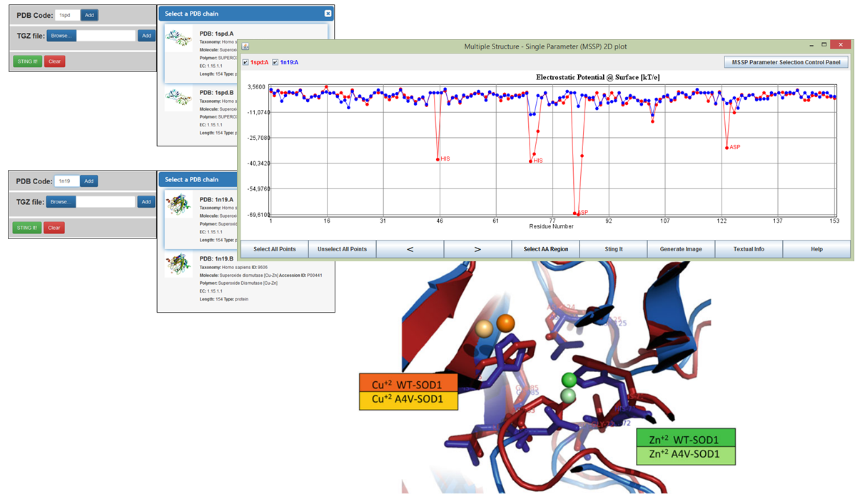
Multiple Structure - Single Parameter (MSSP) 2D plot
MSSP produces a 2D plot of a single protein descriptor for number of structurally aligned protein chains. From a total of 150 protein descriptors available in MSSP, selected out from more than 1500 such parameters stored in STING database, it is possible to create easily readable and highly informative XY-plots, where X-axis represents the amino acid position in the multiple structural alignment, and Y-axis represents the descriptor's numerical values. The structures are globally aligned using the structural alignment software: Matching Molecular Models Obtained from Theory (MAMMOTH-mult). MSSP alows the direct comparison of changes in specific descriptors caused by amino acid mutations, relative to the wild type protein.
STING_DB is composed of structural, sequence, function and stability parameters/descriptor for protein analysis. This database operates with a collection of both publicly available data (PDB, HSSP, Prosite) and its own data (contacts, interface contacts, surface accessibility). STING_DB is one of the best known databases of structural parameters reported in per-residue fashion with over 300 of them compiled at a single site.
Under construction.
Under construction.
Under construction.
Contacts Distance Maps (CDM) is a STING's module. It is designed to display graphically all the protein’s contacts. Moreover, the Secondary Structure (SS) elements are also shown in a single line, facilitating theirs visualization for each residue, and contour curves distances maps involving a carbon, ß carbon and LHA-LHA (Least Heavy Atom) are presented in a Java interactive interface.
In STING_PCD users can obtain a complete comparison report of the intrachain interactions for any two chains described in the PDB format file. The user must supply any two PDB ids and corresponding chain ids for the analysis. At the output, a user will receive a list of interactions which were preserved in both chains as well as the list of those which are present in only one of them. Users can also analyse a wild type protein and a corresponding mutant structure with a single point mutantion; in this case a user needs to supply at the input, the mutated amino acid name and the number.
STING_TopSiMap is a module which makes possible to compare the contact maps of two chains in terms of the preserved interactions as well as the ones which are present in only one of the two chains analysed. Users can see / print the images of the maps and also view the contacts in a JMol window where STING presents two structurally aligned chains. Users can also compare the chains in terms of the contacts classification (hydrophobic, aromatic stacking, hydrogen bonds, salt bridges and cysteine bridges) and corresponding energies.
Under construction.
Under construction.
Under construction.
|
Go to Quick Learn:
Basic
Commands
|
Go to Quick Learn:
Modes
|